Coaches and practitioner in both team and individual sports aim to individualize the intensity of both low and high-intensity interval (HIIT) training. In endurance sports, the exercise intensity of HIIT is often prescribed using a percentage/proportion of determined thresholds (i.e. lactate/ventilatory thresholds, critical power/speed, functional threshold power). Furthermore, the maximal aerobic power output/speed (i.e. power output/speed at VO
2max) has developed into the most popular reference point for both setting and monitoring the intensity of HIIT across the sports science literature (e.g. (
1)). As nicely illustrated in Figure 1 by Buchheit and Laursen (
2), two athletes with a similar running speed at VO
2max can have significantly different sprint speeds. If the intensity of a short duration HIIT session is exclusively based on an ‘aerobic marker’ (e.g. intervals at a certain percentage of maximal aerobic speed) the athlete with the higher maximal sprint speed winds up working at a lower percentage of their maximal capacity. This often leads to athletes performing HIIT at different physiological demands and exercise tolerance than expected (
2).
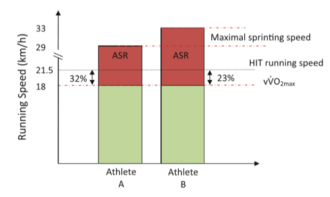
Figure 1. Two athletes with a similar running speed at VO2max can have significantly different sprint speeds. Figure from Buchheit & Laursen (2).
Ideally, exercise intensity for HIIT, particularly within the short duration HIIT domain, should be individualized using a combination of aerobic and anaerobic capacity parameters, in order to have the same training impact among different individuals. What’s becoming clearer now is that we are all wired differently in terms of our aerobic and anaerobic abilities (
2,
3,
7), so we need to strive for better ways at defining this in our athletes if we are to help individuals reach their performance potential.
Defining the Anaerobic Power/Speed Reserve
In runners, the anaerobic speed reserve (ASR) is typically defined as the difference between maximal sprinting speed (MSS) and running speed at VO
2max. In cyclists, the anaerobic power reserve (APR) is defined as the difference between maximal sprint power output and power output at VO
2max. Notwithstanding the important contribution of the neuromuscular system (
4), the APR/ASR range may broadly reflect a combination of both maximal aerobic and anaerobic energetic capacities. Traditionally, this upper range is less appreciated. However more recent data suggests it may be of great use for coaches to individualize exercise intensity of (supramaximal) HIIT.
Calculating Speed/Power Output-Duration Decrement
Studies have used the anaerobic speed/power reserve range to set the minimal and maximal values of a (‘supramaximal’) power-duration or speed-duration curve, typically across a duration between 5 – 300 s (
3,
6-8). Using cycling (i.e. power output) as an example, the following formula describes the decrement in power output over time (
8):
POt = POaer + (POsp – POaer) * e(-k*t)
where
t is the duration of the all-out trial, PO
t is the power output maintained for that trial with a duration of
t, PO
aer is the maximal aerobic power output, PO
sp is the maximal sprint peak power output and
k is the exponent that describes the decrement in power output over time (originally proposed as
k = 0.026 (
8)). This formula aims to predict the power output an athlete can sustain within their anaerobic reserve for all-out efforts lasting from a few seconds to a few minutes. The model assumes that the exponential decrement in all-out speed/power output in relation to duration is similar for different athletes in relation to their ASR/APR. (For more information behind the formula and how the exponent was derived, refer to pioneering papers on these concepts by Weyand, Bundle and colleagues (
3,
4,
7,
8).)
The APR in professional cycling
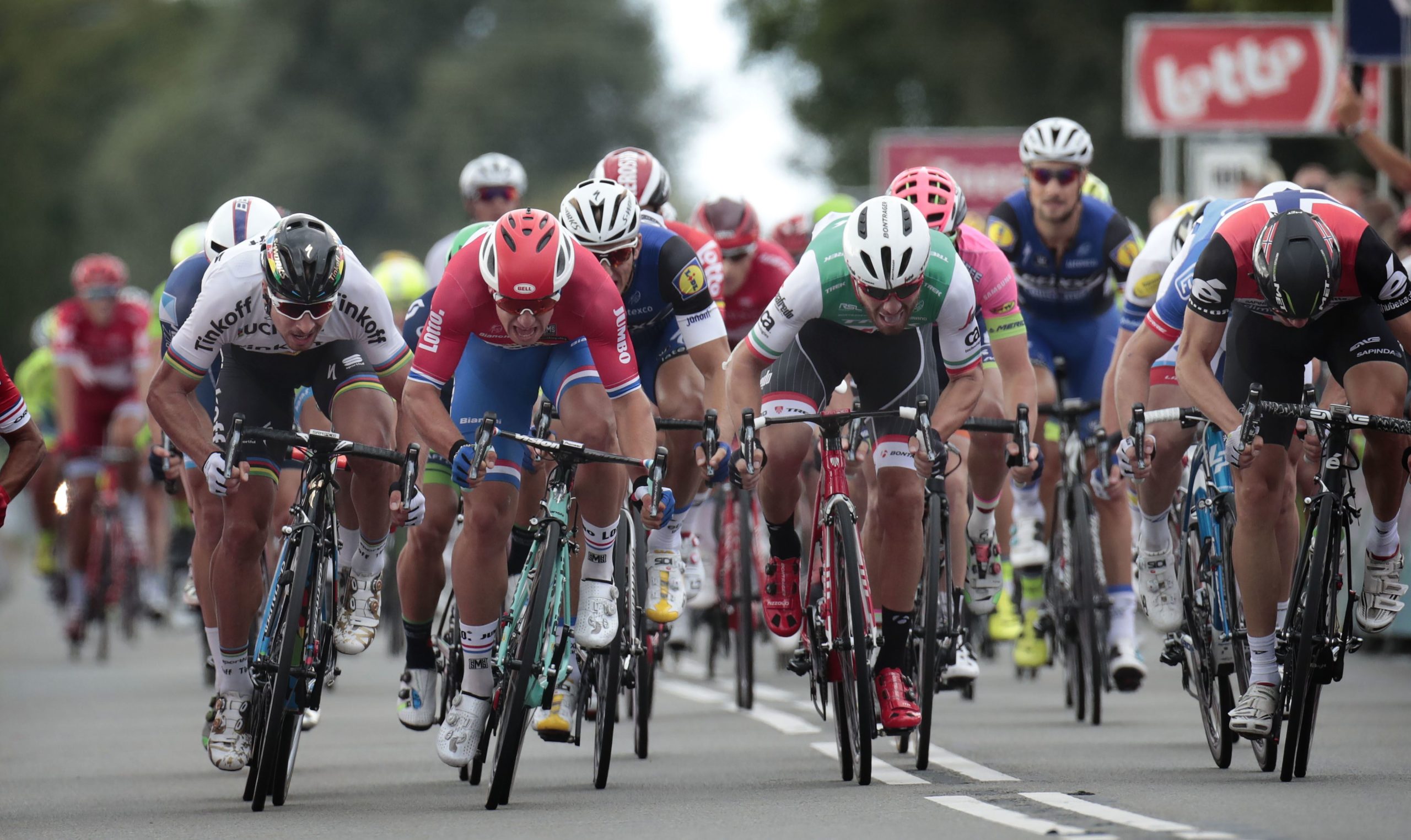
Photo credit: Dion Kerckhoffs/Cor Vos © 2016 motard Jos Verschuur
To explore this concept in professional cycling, we conducted a preliminary pilot study to evaluate how the APR model could predict all-out efforts varying between 10 – 120 s in four professional cyclists (
6). It was shown (Figure 2) that the power output predicted by the model was very largely to nearly perfectly correlated to the actual power output obtained during all-out time trials for each cyclist (r = 0.88 – 0.97) and power output during the all-out trials remained within an average of 6.6% (53 W) of the predicted power output by the model. Even though there were some individual differences in predictive ability (e.g. figure B versus figure D), the results were promising.
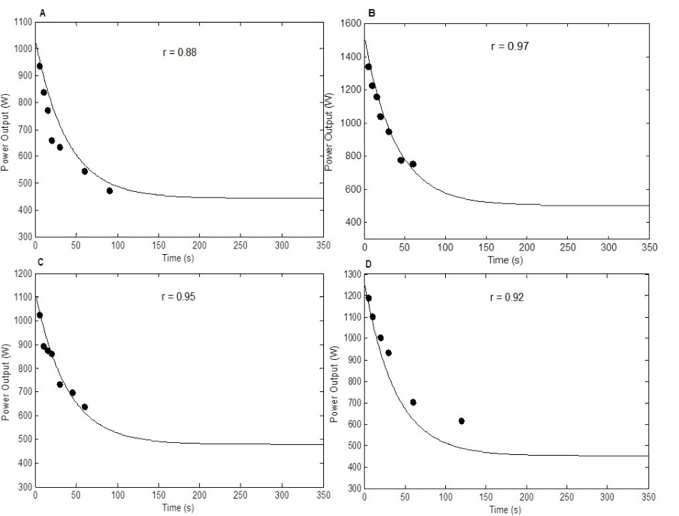
Figure 2: Figure from Sanders et al. (6) showing the power duration curves for participant 1 (A), 2 (B), 3 (C), and 4 (D) when comparing predicted power outputs (line) with the all-out trials (black circles).
While these were exciting results, there were still a few questions that remained unanswered. For example, how well the model would fit across a larger group of (elite) cyclists was still unknown. To evaluate this, I was lucky enough to collaborate with Mathieu Heijboer (Head of Performance at Team LottoNL-Jumbo) and explored the concept of the anaerobic reserve in professional cycling to a greater extent – the paper
now published in the
Journal of Sports Sciences. Similar to our preliminary study, the APR model was able to predict maximal power outputs over durations between 5 – 180 s with reasonable accuracy (Figure 3). Mean deviation between actual and predicted power output was 43 W and 5.9%, slightly better than our first study. While a mean deviation of 43 W might be considered a large margin when the aim is to accurately prescribe training, it must be noted that the power outputs predicted within this short-duration range are in the extreme upper domain (i.e. ~ 450 – 1400 W).

Figure 3: Figure from Sanders et al. (5) record power outputs achieved during training and competition versus those predicted by the APR model. (Dashed line shows the line where actual power output is equal to predicted power output.)
As the model was only able to predict actual versus predicted power output within ~5%, optimizing the predictive ability needs to be an important focus of research in the area in the short term. Nevertheless, the advantages of the model remain promising. For both running and cycling, the lower and upper bound limits of the anaerobic reserve can be determined using two (rather simple) field tests. Subsequently, using the APR/ASR model, a speed or power output-duration curve can be established for each athlete individually. Hence, using the APR model, we can predict record power output over the interval durations before programming HIIT based on a certain proportion of that predicted power output. This may be especially helpful when the aim is to keep a steady performance over each interval (i.e. avoiding the typical fall in power output across first and last interval due to fatigue). Also, when aiming to individualising HIIT sessions across a team, such an approach could prove valuable.
Case study
Taking cycling as the example again – let’s say we are working with a professional cyclist that is preparing for a hilly one-day race. The race is characterised by short hills of durations varying from 60 to 180 s and the coach wants to implement specific intervals at these durations to prepare the cyclist for the demands of the race. For this particular cyclist we established a maximal aerobic power output of 450 W and a maximal sprint power output of 1350 W. (Both measures can be based on laboratory testing (
8) or assessed using a field-based approach (
5,
6).) Using the exponential decay formula (
8), we are able to determine a power output-duration curve ranging between ~5 to 300 s (Figure 4).
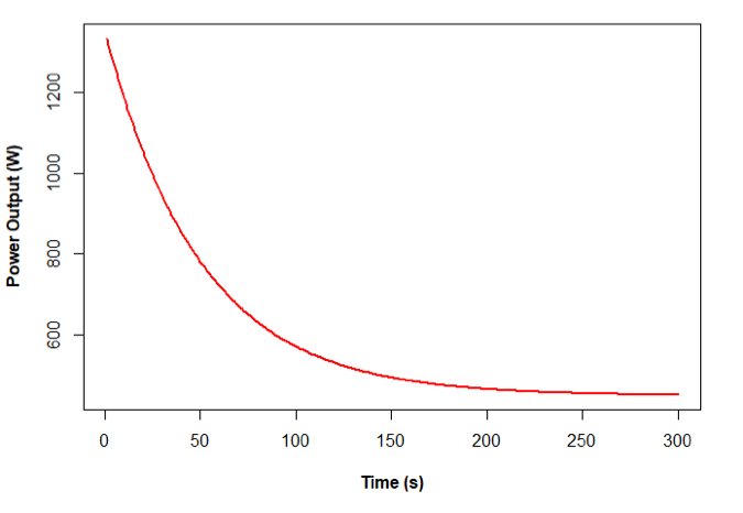
Figure 4: Predicted power duration curve for the professional cyclist with a maximal aerobic power output of 450 W and a maximal sprint peak power output of 1350 W.
Based on the power-duration curve, the power output over 60, 90 and 120 was predicted to be 639 W, 537 W and 490 W, respectively. Depending on the goal of the session, this information can subsequently be used in the prescription of the intensity of the specific intervals. For example, the coach can provide the athlete with a range around the ‘predicted’ power output that he/she should aim for, for example 620 – 650 W, 525 – 550 W, 475 – 500 W for 60, 90 and 120 s intervals, respectively. Another approach could be to use the predicted maximal power output for a given duration (e.g. 639 W for 60 s) and subsequently prescribe interval sessions on a given percentage of that duration (e.g. intervals of ~640 W for 45 s with multiple repetitions). Importantly, the coach/practitioner should always consider individual differences in power output-duration decrement. Feedback from the athlete (e.g. “intervals were too easy”) could prove useful at this stage to monitor if the exponent used within the model should be adjusted. More discussion around the considerations/limitations of this approach can be read in our latest study (
5).
Take-home-point
Since the early studies by Weyand, Bundle and colleagues on the anaerobic reserve and speed/power-duration decrement (
3,
4,
7,
8), more and more studies are examining the practical application of these concepts to (elite) sports performance. I believe that one of the most important take-away points from some of these studies is that integrating both a measure of aerobic and anaerobic capacity when prescribing intensity for HIIT is essential to individualise training intensity and demand, especially for short(er) duration intervals. Further examples on this topic can be found on the
30-15IFT blog. Finally, more research is needed to explore ways of using the anaerobic speed/power reserve to inform training practice. (Some encouraging work by
Gareth Sandford and colleagues is currently shedding more light on these issues in the context of
middle distance running, see
here.) In the meantime, using markers to determine the anaerobic speed/power reserve with the exponential decay formulas might be an additional tool in the toolbox used for prescribing training sessions – but its usage will, as always, depend on the
context and environment it is applied to.
About the author
Dajo Sanders is currently a sport scientist at the University of Stirling, where he coordinates and provides applied sport science support to the scholarship sport programmes. He is passionate about cycling, having previously competed as a road cyclist, and has worked on sport science support projects with multiple professional cycling teams. You can follow him on twitter @DajoSanders
References
- Billat LV. Interval training for performance: a scientific and empirical practice. Special recommendations for middle- and long-distance running. Part II: anaerobic interval training. Sports Med 31: 75-90, 2001.
- Buchheit M and Laursen PB. High-intensity interval training, solutions to the programming puzzle: Part I: cardiopulmonary emphasis. Sports Med 43: 313-338, 2013.
- Bundle MW, Hoyt RW, and Weyand PG. High-speed running performance: a new approach to assessment and prediction. J Appl Physiol (1985) 95: 1955-1962, 2003.
- Bundle MW and Weyand PG. Sprint exercise performance: does metabolic power matter? Exerc Sport Sci Rev 40: 174-182, 2012.
- Sanders D and Heijboer M. The Anaerobic Power Reserve and its Applicability in Professional Road Cycling. J Sports Sci, 2018. [Epub Ahead of Print].
- Sanders D, Heijboer M, Akubat I, Meijer K, and Hesselink MK. Predicting High-Power Performance in Professional Cyclists. Int J Sports Physiol Perform 12: 410-413, 2017.
- Weyand PG and Bundle MW. Energetics of high-speed running: integrating classical theory and contemporary observations. Am J Physiol Regul Integr Comp Physiol 288: 956-965, 2005.
- Weyand PG, Lin JE, and Bundle MW. Sprint performance-duration relationships are set by the fractional duration of external force application. Am J Physiol Regul Integr Comp Physiol 290: 758-765, 2006.